Plant segmentation
Phenotyping is important to plant science because of its applications in breeding and crop management. It relies on leaf detection and leaf segmentation. This is because leaf color is used to estimate nutritional status, while area index is used to measure plant growth and estimate final yield. In this tutorial, we illustrate the use of JustDeepIt to train U2-Net[1] and apply the trained model to leaf segmentation.
Dataset preparation
The dataset used in this case study can be downloaded from Computer Vision Problems in Plant Phenotyping CVPPP (CVPPP 2017 Challenges). The dataset is intended for developing and evaluating methods for plant detection, localization, segmentation, and other tasks. The original dataset is grouped into three levels: ray, stack, and plant. Level tray contains images of trays, including multiple plants compiled by annotations, while levels stack and plant contain images of a single plant, with the former containing stacks and the latter containing only plants. In this study, we use the images at level tray for training and plant segmentation.
The dataset contains 27 tray-level images with filenames ara2013_tray*_rgb.png
where * represents digits from 01 to 27.
We create folders trains, masks, and tests
in the workspace (PPD2013) to store the training, mask, and test images, respectively.
We copy four images with the corresponding masks, tray01, tray09, tray18, and tray27,
into folder trains and masks, respectively;
and then copy all the images without masks into folder tests.
Note that the training and mask images should be the same name under the different folders.
Here, for example, we (i) rename the image ara2013_tray01_rgb.png to ara2013_tray01.png and
put the image into the trains folder
and (ii) rename the mask ara2013_tray01_fg.png to ara2013_tray01.png and
put the mask into the masks folder.
The above dataset preparation can be performed manually or automatically using the following shell scripts:
# download tutorials/PPD2013 or clone JustDeepIt repository from https://github.com/biunit/JustDeepIt
git clone https://github.com/biunit/JustDeepIt
cd JustDeepIt/tutorials/PPD2013

# download dataset (Plant_Phenotyping_Datasets.zip) from http://www.plant-phenotyping.org/datasets
# and put Plant_Phenotyping_Datasets.zip in JustDeepIt/tutorials/PPD2013

# decompress data
unzip Plant_Phenotyping_Datasets.zip

# create folders to store images for training and inference
mkdir -p trains
mkdir -p masks
mkdir -p tests

# select 4 images and the corresponding mask images for training
cp Plant_Phenotyping_Datasets/Tray/Ara2013-Canon/ara2013_tray01_rgb.png trains/ara2013_tray01.png
cp Plant_Phenotyping_Datasets/Tray/Ara2013-Canon/ara2013_tray09_rgb.png trains/ara2013_tray09.png
cp Plant_Phenotyping_Datasets/Tray/Ara2013-Canon/ara2013_tray18_rgb.png trains/ara2013_tray18.png
cp Plant_Phenotyping_Datasets/Tray/Ara2013-Canon/ara2013_tray27_rgb.png trains/ara2013_tray27.png
cp Plant_Phenotyping_Datasets/Tray/Ara2013-Canon/ara2013_tray01_fg.png masks/ara2013_tray01.png
cp Plant_Phenotyping_Datasets/Tray/Ara2013-Canon/ara2013_tray09_fg.png masks/ara2013_tray09.png
cp Plant_Phenotyping_Datasets/Tray/Ara2013-Canon/ara2013_tray18_fg.png masks/ara2013_tray18.png
cp Plant_Phenotyping_Datasets/Tray/Ara2013-Canon/ara2013_tray27_fg.png masks/ara2013_tray27.png

# use all images for inference
cp Plant_Phenotyping_Datasets/Tray/Ara2013-Canon/*_rgb.png tests/
Settings
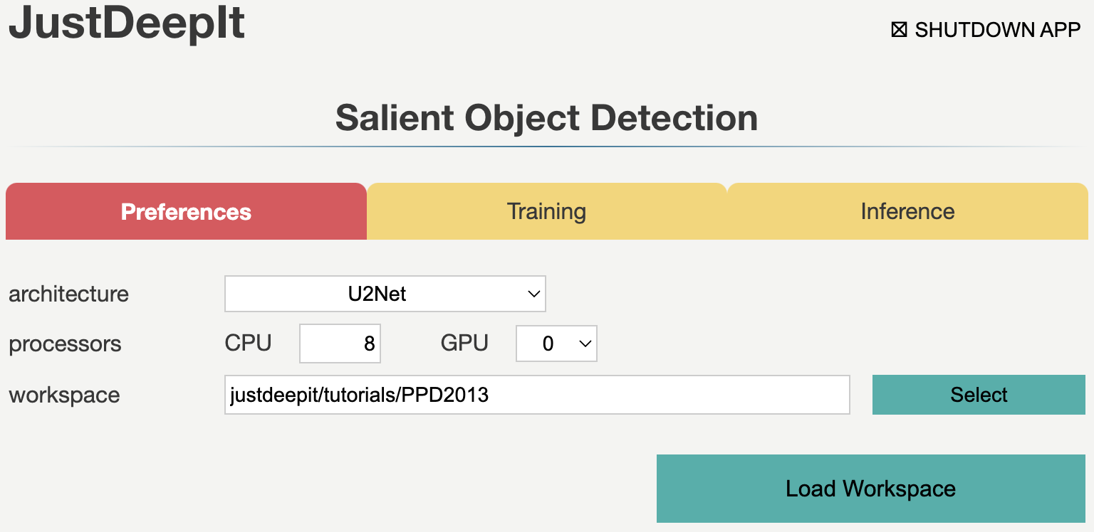
To start JustDeepIt, we open the terminal and run the following command. Then, we open the web browser, access to http://127.0.0.1:8000, and start “Salient Object Detection” mode.
justdeepit
# INFO:uvicorn.error:Started server process [61]
# INFO:uvicorn.error:Waiting for application startup.
# INFO:uvicorn.error:Application startup complete.
# INFO:uvicorn.error:Uvicorn running on http://127.0.0.1:8000 (Press CTRL+C to quit)
We set the workspace to the location containing folders
trains, masks, and tests,
and press Load Workspace button.
Note that the value of workspace may be different from
the screenshot below depending on user’s environment.
After loading workspace, the functions of the Training and Inference become available.
Trainig
To train the model,
we select tab Training
and specify model weight as the location to store the training weight,
image folder as the folder containing training images (i.e., trains)
and annotation as the folder containing mask images (i.e., masks).
The other parameters are set as shown in the screenshot below.
Note that the values of model weight, image folder, and annotation may be different
from the screenshot depending on user’s environment.
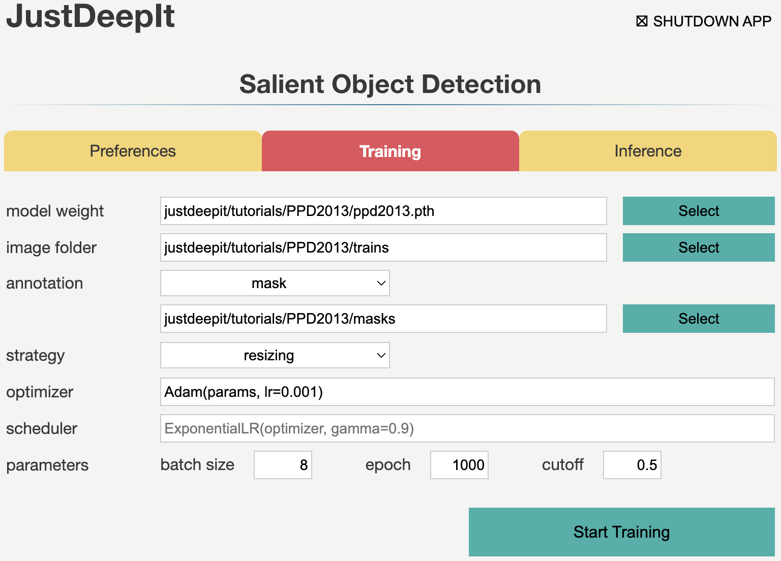
As the images in this dataset have a resolution of 3108 x 2324 pixels and each image contains 24 plants, the training images are large and capture many small objects. Thus, random cropping strategy is the suitable selection for training (see Training Strategy for details). Here we set JustDeepIt to crop areas of 320 x 320 pixels for training. As random cropping is applied once per image and epoch and only four training images were available, we require many epochs (1,000 epochs in this case study) for training to ensure a high detection performance. After setting the parameters as in the screenshot below, we press Start Training button to start model training.
Inference
In tab Inference,
we specify model weight to the training weights,
whose file usually has extension .pth,
image folder as the folder containing images for detection (i.e., tests),
and the other parameters as shown in the screenshot below.
The values of model weight and image folder may be different
from the screenshot depending on user’s environment.
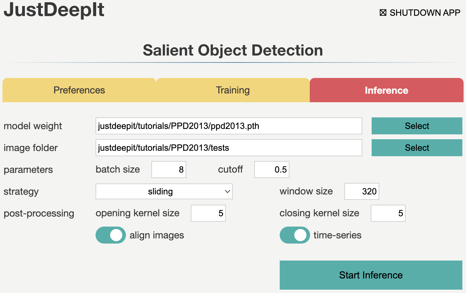
Note that, to summarize objects over time, we activate option time-series. In addition, to align plants in each image through time-series by location, we activate option align images. In addition, as we trained the model on areas of 320 x 320 pixels that were randomly cropped from the original image, we also need input of the same size and scale for the model to ensure the high detection performance. Thus, during detection, we use the sliding approach (see Detection Strategy for details) to crop areas of 320 x 320 pixels from the top left to the bottom right of the original image, performe salient object detection for all the areas, and finally merge the detection results into a single image.
Then, we press Start Inference button to perform salient object detection (i.e., plant segmentation). The results of prediction and summarization were saved in the workspace as specified in tab Preferences.
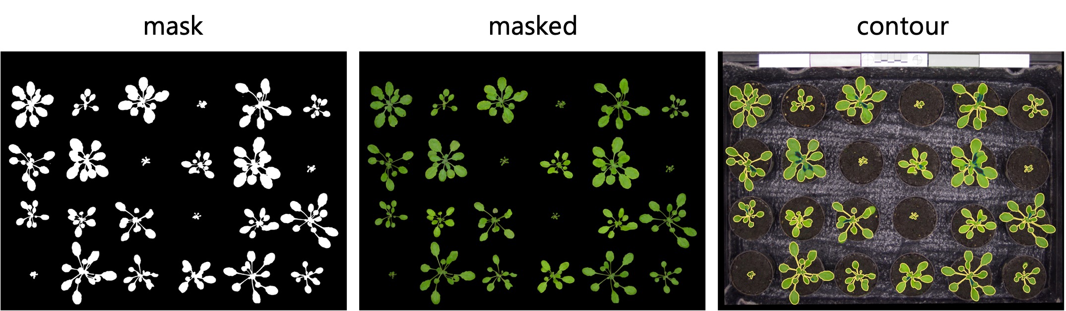
JustDeepIt generates three types of images: mask, masked, and contour during the inference process, as respectively shown in the images below.
Downstream analyses
The time-series images can be aligned to generate videos using third-party software such as ffmpeg command, free GUI software, and online service.
Further, the identification of each object (each plant in this case) is automatically assigned over time, as shown in the image below. Hence, the same identifier is assigned to objects that are almost at the same position across the images. This is because we turned on time-series and align images option during detection processes. In this case study, 27 images containing 24 plants per image are used, and thus the detected objects are identified from 1 to 24.
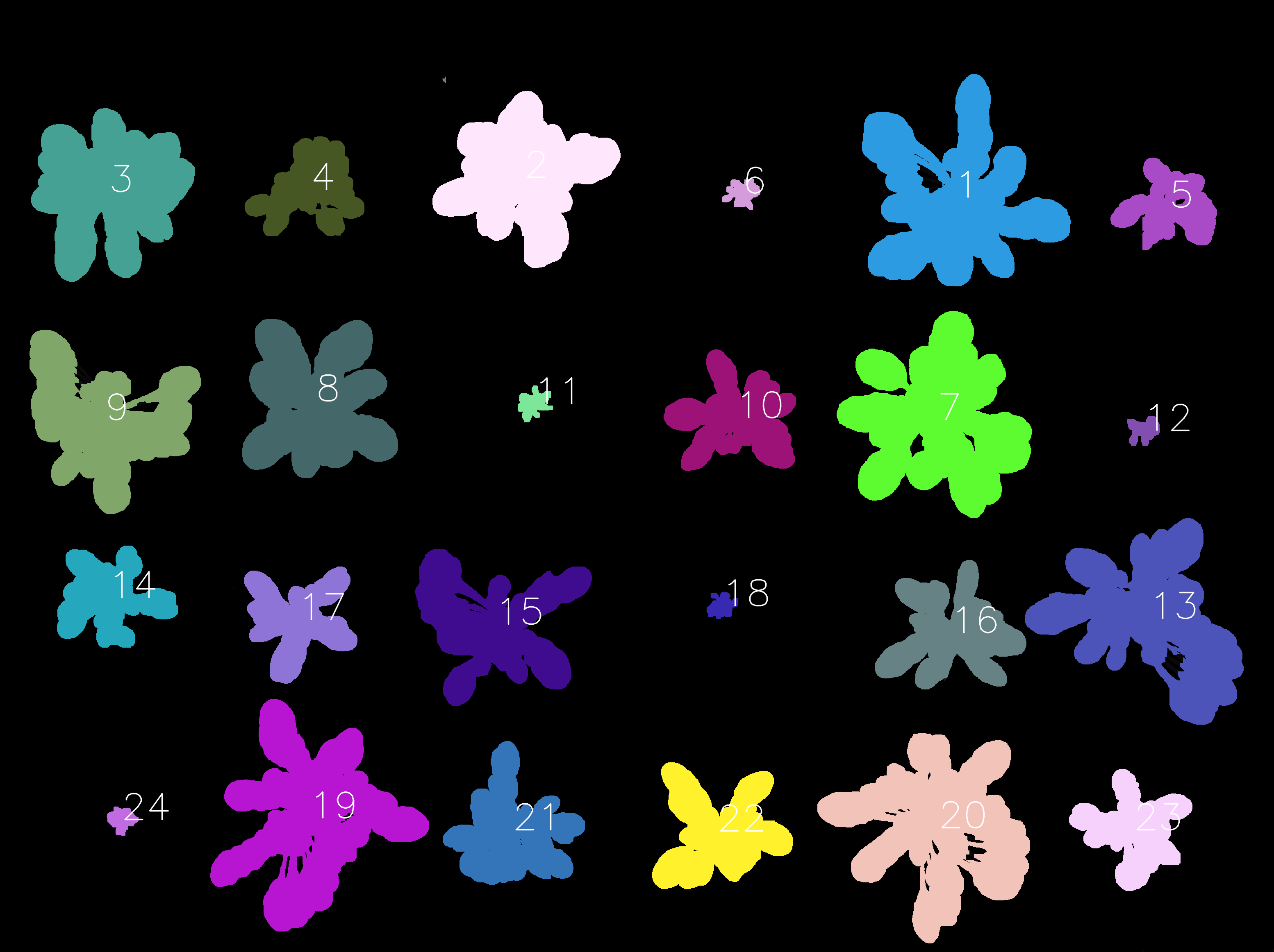
Information about each object,
such as the coordinates of center position, radius, size, and color in RGB, HSV, and L*a*b* color spaces
will be recorded in *.objects.tsv files in the workspace justdeepitws/outputs folder.
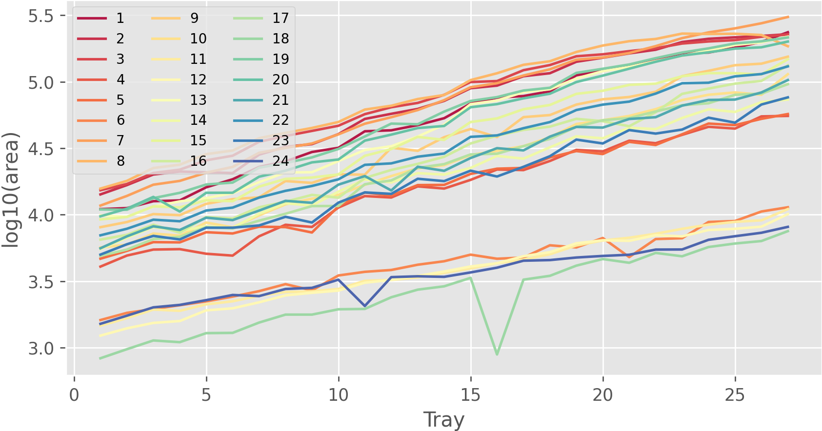
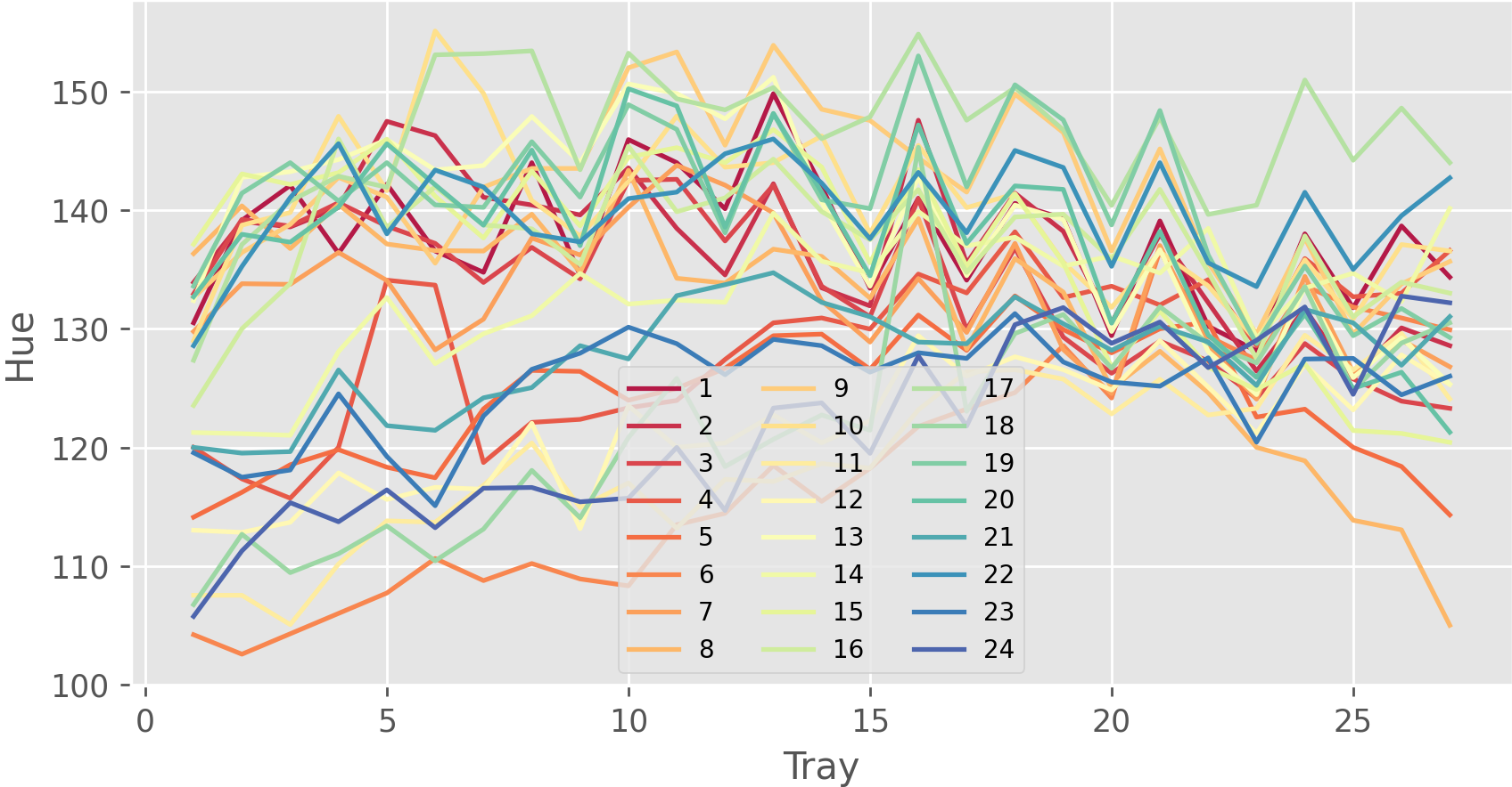
Python or R can be used to visualize summarization results,
such as the projected area of each plant and the color of each plant over time.